This is not Fake News (Fact)

Rampant misinformation—often called “fake news”—is one of the defining features of contemporary democratic life. In this Blog Post, we will develop and assess a fake news classifier using Tensorflow.

Data Source

Our data for this assignment comes from the article

Ahmed H, Traore I, Saad S. (2017) “Detection of Online Fake News Using N-Gram Analysis and Machine Learning Techniques. In: Traore I., Woungang I., Awad A. (eds) Intelligent, Secure, and Dependable Systems in Distributed and Cloud Environments. ISDDC 2017. Lecture Notes in Computer Science, vol 10618. Springer, Cham (pp. 127-138).

§1. Import Packages

The following imports are required to follow along with this post.

import numpy as np
import pandas as pd
import tensorflow as tf
import re
import string

import nltk
from nltk.corpus import stopwords

from tensorflow.keras import layers, losses, utils
from tensorflow import keras

from tensorflow.keras.layers.experimental.preprocessing import TextVectorization

from sklearn.decomposition import PCA

from matplotlib import pyplot as plt

# for embedding viz
import plotly.express as px 
import plotly.io as pio
pio.templates.default = "plotly_white"

§2. Acquire Training Data

To begin, we download the training data and examine what it looks like.

url = "https://github.com/PhilChodrow/PIC16b/blob/master/datasets/fake_news_train.csv?raw=true"
df = pd.read_csv(url)

df.head()

	Unnamed: 0	title	text	fake
0	17366	Merkel: Strong result for Austria's FPO 'big c...	German Chancellor Angela Merkel said on Monday...	0
1	5634	Trump says Pence will lead voter fraud panel	WEST PALM BEACH, Fla.President Donald Trump sa...	0
2	17487	JUST IN: SUSPECTED LEAKER and “Close Confidant...	On December 5, 2017, Circa s Sara Carter warne...	1
3	12217	Thyssenkrupp has offered help to Argentina ove...	Germany s Thyssenkrupp, has offered assistance...	0
4	5535	Trump say appeals court decision on travel ban...	President Donald Trump on Thursday called the ...	0

Each row of the data corresponds to an article. The title column gives the title of the article, while the text column gives the full article text. The final column, called fake, is 0 if the article is true and 1 if the article contains fake news, as determined by the authors of the paper above.

§3. Make Dataset

Next, we will write a function called make_dataset. This function should do two things:

Remove stopwords from the article text and title. A stopword is a word that is usually considered to be uninformative, such as “the,” “and,” or “but.”
Construct and return a tf.data.Dataset with two inputs and one output. The input should be of the form (title, text), and the output should consist only of the fake column.

# Download stop words nltk data
nltk.download('stopwords')

def make_dataset(df):
    """ 
    Creates a Tensorflow Dataset from a Pandas DataFrame with 'fake news' data.
    
    Args:
        df (DataFrame): Contains title, text, and label for each article.

    Returns:
        Dataset: Contains title, text, and label for each article.
    """
    stop = stopwords.words('english')

    # Exclude stopwords with Python's list comprehension and pandas.DataFrame.apply.
    df['title'] = df['title'].apply(lambda x: ' '.join([word for word in x.split() if word not in (stop)]))
    df['text'] = df['text'].apply(lambda x: ' '.join([word for word in x.split() if word not in (stop)]))

    data = tf.data.Dataset.from_tensor_slices(
        ({'title': df[['title']], 'text': df[['text']]},
        {'fake' : df[['fake']]})
    )
    
    return data

# Create a Dataset with a batch size of 100.
data = make_dataset(df).batch(100)

Validation Data

Now that we have constructed the primary Dataset, we split of 20% of it to use for validation.

# Randomize the order of the data.
data = data.shuffle(buffer_size = len(data))

train_size = int(0.8*len(data))

train = data.take(train_size)
val = data.skip(train_size)

print(len(train), len(val))

180 45

Base Rate

Let’s compute the base rate of the data.

sum(df['fake'])/len(df)

0.522963160942581

If the model always predicted 1, it would have an accuracy of ~52%.

TextVectorization

Now we want to prepare a text vectorization layer for use in our models.

#preparing a text vectorization layer for tf model
size_vocabulary = 2000

def standardization(input_data):
    lowercase = tf.strings.lower(input_data)
    no_punctuation = tf.strings.regex_replace(lowercase,
                                  '[%s]' % re.escape(string.punctuation),'')
    return no_punctuation 

title_vectorize_layer = TextVectorization(
    standardize=standardization,
    max_tokens=size_vocabulary, # only consider this many words
    output_mode='int',
    output_sequence_length=500) 

title_vectorize_layer.adapt(train.map(lambda x, y: x["title"]))

text_vectorize_layer = TextVectorization(
    standardize=standardization,
    max_tokens=size_vocabulary, # only consider this many words
    output_mode='int',
    output_sequence_length=500) 

text_vectorize_layer.adapt(train.map(lambda x, y: x["text"]))

§4. Create Models

Now, lets create Tensorflow models that can offer a perspective on the following question:

When detecting fake news, is it most effective to focus on only the title of the article, the full text of the article, or both?

First Model

In the first model, we will only use the article title as an input.

title_input = keras.Input(
    shape = (1,),
    name = 'title',
    dtype = 'string'
)

title_features = title_vectorize_layer(title_input)

# Create an embedding layer that can be used with both title and text inputs.
embedding_layer = layers.Embedding(size_vocabulary, output_dim=10, name='embedding')

# Layers specific to this model.
title_features = embedding_layer(title_features)
title_features = layers.Dropout(0.2)(title_features)
title_features = layers.GlobalAveragePooling1D()(title_features)
title_features = layers.Dropout(0.2)(title_features)
title_features = layers.Dense(32, activation='relu')(title_features)

#Create an output layer that can be used for all of the models.
output_layer = layers.Dense(2, name='fake')
output = output_layer(title_features)

model1 = keras.Model(
    inputs = title_input,
    outputs = output
)

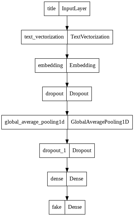
model1.summary()

Model: "model"
_________________________________________________________________
 Layer (type)                Output Shape              Param #   
=================================================================
 title (InputLayer)          [(None, 1)]               0         
                                                                 
 text_vectorization (TextVec  (None, 500)              0         
 torization)                                                     
                                                                 
 embedding (Embedding)       (None, 500, 10)           20000     
                                                                 
 dropout (Dropout)           (None, 500, 10)           0         
                                                                 
 global_average_pooling1d (G  (None, 10)               0         
 lobalAveragePooling1D)                                          
                                                                 
 dropout_1 (Dropout)         (None, 10)                0         
                                                                 
 dense (Dense)               (None, 32)                352       
                                                                 
 fake (Dense)                (None, 2)                 66        
                                                                 
=================================================================
Total params: 20,418
Trainable params: 20,418
Non-trainable params: 0
_________________________________________________________________

utils.plot_model(model1)

png

model1.compile(optimizer = "adam",
              loss = losses.SparseCategoricalCrossentropy(from_logits=True),
              metrics=['accuracy']
)

history1 = model1.fit(train, 
                    validation_data=val,
                    epochs = 20, 
                    verbose = True)

Epoch 1/20


/usr/local/lib/python3.7/dist-packages/keras/engine/functional.py:559: UserWarning: Input dict contained keys ['text'] which did not match any model input. They will be ignored by the model.
  inputs = self._flatten_to_reference_inputs(inputs)


180/180 [==============================] - 2s 6ms/step - loss: 0.6901 - accuracy: 0.5223 - val_loss: 0.6837 - val_accuracy: 0.5176
Epoch 2/20
180/180 [==============================] - 1s 6ms/step - loss: 0.6270 - accuracy: 0.7508 - val_loss: 0.5188 - val_accuracy: 0.9243
Epoch 3/20
180/180 [==============================] - 1s 5ms/step - loss: 0.3783 - accuracy: 0.9312 - val_loss: 0.2633 - val_accuracy: 0.9398
Epoch 4/20
180/180 [==============================] - 1s 5ms/step - loss: 0.2077 - accuracy: 0.9528 - val_loss: 0.1554 - val_accuracy: 0.9658
Epoch 5/20
180/180 [==============================] - 1s 5ms/step - loss: 0.1416 - accuracy: 0.9635 - val_loss: 0.1143 - val_accuracy: 0.9660
Epoch 6/20
180/180 [==============================] - 1s 5ms/step - loss: 0.1108 - accuracy: 0.9699 - val_loss: 0.0950 - val_accuracy: 0.9731
Epoch 7/20
180/180 [==============================] - 1s 5ms/step - loss: 0.0922 - accuracy: 0.9731 - val_loss: 0.0730 - val_accuracy: 0.9778
Epoch 8/20
180/180 [==============================] - 1s 5ms/step - loss: 0.0810 - accuracy: 0.9749 - val_loss: 0.0769 - val_accuracy: 0.9738
Epoch 9/20
180/180 [==============================] - 1s 6ms/step - loss: 0.0714 - accuracy: 0.9784 - val_loss: 0.0623 - val_accuracy: 0.9760
Epoch 10/20
180/180 [==============================] - 1s 6ms/step - loss: 0.0637 - accuracy: 0.9808 - val_loss: 0.0589 - val_accuracy: 0.9807
Epoch 11/20
180/180 [==============================] - 1s 5ms/step - loss: 0.0610 - accuracy: 0.9809 - val_loss: 0.0548 - val_accuracy: 0.9804
Epoch 12/20
180/180 [==============================] - 1s 6ms/step - loss: 0.0557 - accuracy: 0.9815 - val_loss: 0.0417 - val_accuracy: 0.9888
Epoch 13/20
180/180 [==============================] - 1s 6ms/step - loss: 0.0563 - accuracy: 0.9823 - val_loss: 0.0500 - val_accuracy: 0.9862
Epoch 14/20
180/180 [==============================] - 1s 6ms/step - loss: 0.0512 - accuracy: 0.9829 - val_loss: 0.0426 - val_accuracy: 0.9867
Epoch 15/20
180/180 [==============================] - 1s 5ms/step - loss: 0.0488 - accuracy: 0.9848 - val_loss: 0.0342 - val_accuracy: 0.9908
Epoch 16/20
180/180 [==============================] - 1s 5ms/step - loss: 0.0454 - accuracy: 0.9849 - val_loss: 0.0635 - val_accuracy: 0.9816
Epoch 17/20
180/180 [==============================] - 1s 6ms/step - loss: 0.0452 - accuracy: 0.9852 - val_loss: 0.0317 - val_accuracy: 0.9901
Epoch 18/20
180/180 [==============================] - 1s 5ms/step - loss: 0.0413 - accuracy: 0.9869 - val_loss: 0.0314 - val_accuracy: 0.9898
Epoch 19/20
180/180 [==============================] - 1s 5ms/step - loss: 0.0421 - accuracy: 0.9867 - val_loss: 0.0339 - val_accuracy: 0.9898
Epoch 20/20
180/180 [==============================] - 1s 5ms/step - loss: 0.0400 - accuracy: 0.9874 - val_loss: 0.0344 - val_accuracy: 0.9896

def plot_history(hist):
    """ 
    Creates a plot of a model's training and validation accuracies.
    
    Args:
        hist (History): a keras model training history
    """
    plt.plot(hist.history["accuracy"], label = "training")
    plt.plot(hist.history["val_accuracy"], label = "validation")
    plt.gca().set(xlabel = "epoch", ylabel = "accuracy")
    plt.legend()
    plt.show()

plot_history(history1)

png

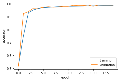
The validation accuracy stabilizes around 99%.

Second Model

In the second model, we will only use the article text as an input.

text_input = keras.Input(
    shape = (1,),
    name = 'text',
    dtype = 'string'
)

text_features = text_vectorize_layer(text_input)
text_features = embedding_layer(text_features)
text_features = layers.Dropout(0.2)(text_features)
text_features = layers.GlobalAveragePooling1D()(text_features)
text_features = layers.Dropout(0.2)(text_features)
text_features = layers.Dense(32, activation='relu')(text_features)
output = output_layer(text_features)

model2 = keras.Model(
    inputs = text_input,
    outputs = output
)

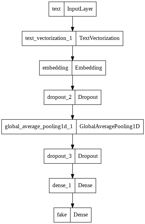
model2.summary()

Model: "model_1"
_________________________________________________________________
 Layer (type)                Output Shape              Param #   
=================================================================
 text (InputLayer)           [(None, 1)]               0         
                                                                 
 text_vectorization_1 (TextV  (None, 500)              0         
 ectorization)                                                   
                                                                 
 embedding (Embedding)       (None, 500, 10)           20000     
                                                                 
 dropout_2 (Dropout)         (None, 500, 10)           0         
                                                                 
 global_average_pooling1d_1   (None, 10)               0         
 (GlobalAveragePooling1D)                                        
                                                                 
 dropout_3 (Dropout)         (None, 10)                0         
                                                                 
 dense_1 (Dense)             (None, 32)                352       
                                                                 
 fake (Dense)                (None, 2)                 66        
                                                                 
=================================================================
Total params: 20,418
Trainable params: 20,418
Non-trainable params: 0
_________________________________________________________________

utils.plot_model(model2)

png

model2.compile(optimizer = "adam",
              loss = losses.SparseCategoricalCrossentropy(from_logits=True),
              metrics=['accuracy']
)

history2 = model2.fit(train, 
                    validation_data=val,
                    epochs = 20, 
                    verbose = True)

Epoch 1/20


/usr/local/lib/python3.7/dist-packages/keras/engine/functional.py:559: UserWarning: Input dict contained keys ['title'] which did not match any model input. They will be ignored by the model.
  inputs = self._flatten_to_reference_inputs(inputs)


180/180 [==============================] - 3s 12ms/step - loss: 0.6704 - accuracy: 0.5866 - val_loss: 0.5883 - val_accuracy: 0.8682
Epoch 2/20
180/180 [==============================] - 2s 11ms/step - loss: 0.5019 - accuracy: 0.8032 - val_loss: 0.3380 - val_accuracy: 0.9204
Epoch 3/20
180/180 [==============================] - 2s 11ms/step - loss: 0.3284 - accuracy: 0.8881 - val_loss: 0.2371 - val_accuracy: 0.9316
Epoch 4/20
180/180 [==============================] - 2s 11ms/step - loss: 0.2476 - accuracy: 0.9178 - val_loss: 0.1732 - val_accuracy: 0.9533
Epoch 5/20
180/180 [==============================] - 2s 11ms/step - loss: 0.2000 - accuracy: 0.9339 - val_loss: 0.1537 - val_accuracy: 0.9596
Epoch 6/20
180/180 [==============================] - 2s 11ms/step - loss: 0.1657 - accuracy: 0.9477 - val_loss: 0.1173 - val_accuracy: 0.9671
Epoch 7/20
180/180 [==============================] - 2s 11ms/step - loss: 0.1475 - accuracy: 0.9533 - val_loss: 0.1163 - val_accuracy: 0.9692
Epoch 8/20
180/180 [==============================] - 2s 11ms/step - loss: 0.1323 - accuracy: 0.9589 - val_loss: 0.0988 - val_accuracy: 0.9749
Epoch 9/20
180/180 [==============================] - 2s 11ms/step - loss: 0.1127 - accuracy: 0.9665 - val_loss: 0.0962 - val_accuracy: 0.9751
Epoch 10/20
180/180 [==============================] - 2s 11ms/step - loss: 0.1078 - accuracy: 0.9667 - val_loss: 0.0929 - val_accuracy: 0.9740
Epoch 11/20
180/180 [==============================] - 2s 11ms/step - loss: 0.1023 - accuracy: 0.9694 - val_loss: 0.0789 - val_accuracy: 0.9771
Epoch 12/20
180/180 [==============================] - 2s 11ms/step - loss: 0.0920 - accuracy: 0.9717 - val_loss: 0.0686 - val_accuracy: 0.9813
Epoch 13/20
180/180 [==============================] - 3s 19ms/step - loss: 0.0858 - accuracy: 0.9739 - val_loss: 0.0680 - val_accuracy: 0.9813
Epoch 14/20
180/180 [==============================] - 2s 11ms/step - loss: 0.0822 - accuracy: 0.9747 - val_loss: 0.0673 - val_accuracy: 0.9816
Epoch 15/20
180/180 [==============================] - 2s 11ms/step - loss: 0.0791 - accuracy: 0.9766 - val_loss: 0.0588 - val_accuracy: 0.9827
Epoch 16/20
180/180 [==============================] - 2s 11ms/step - loss: 0.0720 - accuracy: 0.9784 - val_loss: 0.0547 - val_accuracy: 0.9853
Epoch 17/20
180/180 [==============================] - 2s 11ms/step - loss: 0.0690 - accuracy: 0.9791 - val_loss: 0.0557 - val_accuracy: 0.9844
Epoch 18/20
180/180 [==============================] - 2s 11ms/step - loss: 0.0669 - accuracy: 0.9788 - val_loss: 0.0487 - val_accuracy: 0.9867
Epoch 19/20
180/180 [==============================] - 2s 10ms/step - loss: 0.0647 - accuracy: 0.9796 - val_loss: 0.0505 - val_accuracy: 0.9884
Epoch 20/20
180/180 [==============================] - 2s 11ms/step - loss: 0.0593 - accuracy: 0.9823 - val_loss: 0.0495 - val_accuracy: 0.9871

plot_history(history2)

png

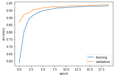
The validation accuracy stabilizes around 99%. This is similar to the title-only model.

Third Model

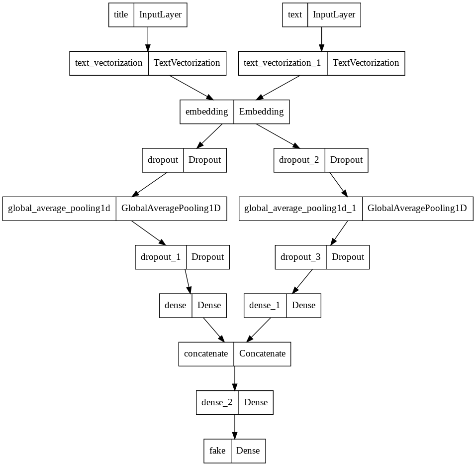
In the third model, we will use both the article title and the article text as input.

# Combine the models to form a new model that takes both text and title inputs.
main = layers.concatenate([title_features, text_features], axis = 1)
main = layers.Dense(32, activation='relu')(main)
output = layers.Dense(2, name='fake')(main)

model3 = keras.Model(
    inputs = [title_input, text_input],
    outputs = output
)

model3.summary()

Model: "model_2"
__________________________________________________________________________________________________
 Layer (type)                   Output Shape         Param #     Connected to                     
==================================================================================================
 title (InputLayer)             [(None, 1)]          0           []                               
                                                                                                  
 text (InputLayer)              [(None, 1)]          0           []                               
                                                                                                  
 text_vectorization (TextVector  (None, 500)         0           ['title[0][0]']                  
 ization)                                                                                         
                                                                                                  
 text_vectorization_1 (TextVect  (None, 500)         0           ['text[0][0]']                   
 orization)                                                                                       
                                                                                                  
 embedding (Embedding)          (None, 500, 10)      20000       ['text_vectorization[0][0]',     
                                                                  'text_vectorization_1[0][0]']   
                                                                                                  
 dropout (Dropout)              (None, 500, 10)      0           ['embedding[0][0]']              
                                                                                                  
 dropout_2 (Dropout)            (None, 500, 10)      0           ['embedding[1][0]']              
                                                                                                  
 global_average_pooling1d (Glob  (None, 10)          0           ['dropout[0][0]']                
 alAveragePooling1D)                                                                              
                                                                                                  
 global_average_pooling1d_1 (Gl  (None, 10)          0           ['dropout_2[0][0]']              
 obalAveragePooling1D)                                                                            
                                                                                                  
 dropout_1 (Dropout)            (None, 10)           0           ['global_average_pooling1d[0][0]'
                                                                 ]                                
                                                                                                  
 dropout_3 (Dropout)            (None, 10)           0           ['global_average_pooling1d_1[0][0
                                                                 ]']                              
                                                                                                  
 dense (Dense)                  (None, 32)           352         ['dropout_1[0][0]']              
                                                                                                  
 dense_1 (Dense)                (None, 32)           352         ['dropout_3[0][0]']              
                                                                                                  
 concatenate (Concatenate)      (None, 64)           0           ['dense[0][0]',                  
                                                                  'dense_1[0][0]']                
                                                                                                  
 dense_2 (Dense)                (None, 32)           2080        ['concatenate[0][0]']            
                                                                                                  
 fake (Dense)                   (None, 2)            66          ['dense_2[0][0]']                
                                                                                                  
==================================================================================================
Total params: 22,850
Trainable params: 22,850
Non-trainable params: 0
__________________________________________________________________________________________________

utils.plot_model(model3)

png

model3.compile(optimizer = "adam",
              loss = losses.SparseCategoricalCrossentropy(from_logits=True),
              metrics=['accuracy']
)

history3 = model3.fit(train, 
                    validation_data=val,
                    epochs = 20, 
                    verbose = True)

Epoch 1/20
180/180 [==============================] - 3s 14ms/step - loss: 0.1706 - accuracy: 0.9832 - val_loss: 0.0270 - val_accuracy: 0.9947
Epoch 2/20
180/180 [==============================] - 2s 12ms/step - loss: 0.0243 - accuracy: 0.9936 - val_loss: 0.0143 - val_accuracy: 0.9960
Epoch 3/20
180/180 [==============================] - 2s 12ms/step - loss: 0.0184 - accuracy: 0.9946 - val_loss: 0.0129 - val_accuracy: 0.9967
Epoch 4/20
180/180 [==============================] - 2s 12ms/step - loss: 0.0143 - accuracy: 0.9955 - val_loss: 0.0094 - val_accuracy: 0.9969
Epoch 5/20
180/180 [==============================] - 2s 12ms/step - loss: 0.0155 - accuracy: 0.9948 - val_loss: 0.0065 - val_accuracy: 0.9976
Epoch 6/20
180/180 [==============================] - 2s 12ms/step - loss: 0.0112 - accuracy: 0.9963 - val_loss: 0.0079 - val_accuracy: 0.9976
Epoch 7/20
180/180 [==============================] - 2s 12ms/step - loss: 0.0096 - accuracy: 0.9968 - val_loss: 0.0037 - val_accuracy: 0.9989
Epoch 8/20
180/180 [==============================] - 2s 12ms/step - loss: 0.0096 - accuracy: 0.9967 - val_loss: 0.0061 - val_accuracy: 0.9976
Epoch 9/20
180/180 [==============================] - 2s 12ms/step - loss: 0.0093 - accuracy: 0.9967 - val_loss: 0.0054 - val_accuracy: 0.9989
Epoch 10/20
180/180 [==============================] - 2s 12ms/step - loss: 0.0080 - accuracy: 0.9975 - val_loss: 0.0056 - val_accuracy: 0.9984
Epoch 11/20
180/180 [==============================] - 2s 12ms/step - loss: 0.0080 - accuracy: 0.9975 - val_loss: 0.0047 - val_accuracy: 0.9989
Epoch 12/20
180/180 [==============================] - 2s 12ms/step - loss: 0.0087 - accuracy: 0.9973 - val_loss: 0.0025 - val_accuracy: 0.9996
Epoch 13/20
180/180 [==============================] - 2s 13ms/step - loss: 0.0068 - accuracy: 0.9978 - val_loss: 0.0012 - val_accuracy: 1.0000
Epoch 14/20
180/180 [==============================] - 2s 12ms/step - loss: 0.0057 - accuracy: 0.9981 - val_loss: 0.0026 - val_accuracy: 0.9993
Epoch 15/20
180/180 [==============================] - 2s 13ms/step - loss: 0.0062 - accuracy: 0.9977 - val_loss: 9.3196e-04 - val_accuracy: 1.0000
Epoch 16/20
180/180 [==============================] - 2s 12ms/step - loss: 0.0053 - accuracy: 0.9984 - val_loss: 0.0026 - val_accuracy: 0.9998
Epoch 17/20
180/180 [==============================] - 2s 12ms/step - loss: 0.0058 - accuracy: 0.9979 - val_loss: 0.0019 - val_accuracy: 0.9998
Epoch 18/20
180/180 [==============================] - 2s 12ms/step - loss: 0.0048 - accuracy: 0.9985 - val_loss: 0.0010 - val_accuracy: 0.9998
Epoch 19/20
180/180 [==============================] - 2s 12ms/step - loss: 0.0050 - accuracy: 0.9986 - val_loss: 9.2361e-04 - val_accuracy: 0.9996
Epoch 20/20
180/180 [==============================] - 2s 12ms/step - loss: 0.0042 - accuracy: 0.9988 - val_loss: 0.0022 - val_accuracy: 0.9996

plot_history(history3)

png

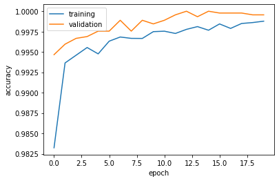
The validation accuracy stabilizes close to 100%. This slightly better than the previous models.

§5. Model Evaluation

Now we’ll test our model performance on unseen test data. For this part, we will use best model, model3, and ignore the other two.

url = "https://github.com/PhilChodrow/PIC16b/blob/master/datasets/fake_news_test.csv?raw=true"
df2 = pd.read_csv(url)

test = make_dataset(df2).batch(100)

loss, accuracy = model3.evaluate(test)
print('Test accuracy :', accuracy)

225/225 [==============================] - 2s 8ms/step - loss: 0.0172 - accuracy: 0.9958
Test accuracy : 0.9957681894302368

The validation accuracy on the test set is also close to 100%. This lines up with the training and validation results. We can conclude that when detecting fake news, is it most effective to focus on both the title and the full text of the article.

§6. Embedding Visualization

Finally, we can create a visualization of the embedding that the model learned.

def get_pca_df(model, vec_layer):
    """ 
    Creates an visualization of the embedding that a model learned.
    
    Args:
        model: Trained model with embedding layer
        vec_layer: TextVectorization() layer used with the model

    Returns:
        embedding_df: DataFrame of word vectors
    """
    # get the weights from the embedding layer
    weights = model.get_layer('embedding').get_weights()[0]

    # get the vocabulary from our data prep for later
    vocab = vec_layer.get_vocabulary()
    pca = PCA(n_components=2)
    weights = pca.fit_transform(weights)

    embedding_df = pd.DataFrame({
        'word' : vocab, 
        'x0'   : weights[:,0],
        'x1'   : weights[:,1]
    })

    return embedding_df

def plot_embedding(model, vec_layer):
    """ 
    Creates an visualization of the embedding that a model learned.
    
    Args:
        model: Trained model with embedding layer
        vec_layer: TextVectorization() layer used with the model

    Returns:
        fig: Plotly scatter plot of word vectors
    """
    df = get_pca_df(model, vec_layer)

    fig = px.scatter(df, 
                     x = "x0", 
                     y = "x1", 
                     size = [2]*len(df),
                     opacity = 0.5,
                     hover_name = "word")
    
    fig.update_traces(marker=dict(line=dict(width=0)),
                      selector=dict(mode='markers'))

    return fig

Let’s use the vocab from the article text.

fig = plot_embedding(model3, text_vectorize_layer)
fig.show()

Based on this plot, words relating to politics such as “gop”, “hillary”, and “terrorists”, along with words such as “truth”, “true”, and “lying” are good indicators of fake news as they have similarly negative x1 values.

Written on May 15, 2022