
Dog or Not-Dog (Cat)
In this blog post, we will create several neural network models in order to distinguish between images of cats and dogs. We will work incrementally, implementing new techniques at each step to make improvements.
Acknowledgment
Major parts of this Blog Post assignment, including several code chunks, are based on the TensorFlow Transfer Learning Tutorial. You may find that consulting this tutorial is helpful while completing this assignment, although this shouldn’t be necessary.
§1. Load Packages and Obtain Data
To follow this tutorial, the following imports are required.
import os
import tensorflow as tf
from tensorflow.keras import utils, layers, models
from matplotlib import pyplot as plt
Now, let’s access the data. We’ll use a sample data set provided by the TensorFlow team that contains labeled images of cats and dogs.
# location of data
_URL = 'https://storage.googleapis.com/mledu-datasets/cats_and_dogs_filtered.zip'

# download the data and extract it
path_to_zip = utils.get_file('cats_and_dogs.zip', origin=_URL, extract=True)

# construct paths
PATH = os.path.join(os.path.dirname(path_to_zip), 'cats_and_dogs_filtered')

train_dir = os.path.join(PATH, 'train')
validation_dir = os.path.join(PATH, 'validation')

# parameters for datasets
BATCH_SIZE = 32
IMG_SIZE = (160, 160)

# construct train and validation datasets
train_dataset = utils.image_dataset_from_directory(train_dir,
                                                   shuffle=True,
                                                   batch_size=BATCH_SIZE,
                                                   image_size=IMG_SIZE)

validation_dataset = utils.image_dataset_from_directory(validation_dir,
                                                        shuffle=True,
                                                        batch_size=BATCH_SIZE,
                                                        image_size=IMG_SIZE)

# construct the test dataset by taking every 5th observation out of the validation dataset
val_batches = tf.data.experimental.cardinality(validation_dataset)
test_dataset = validation_dataset.take(val_batches // 5)
validation_dataset = validation_dataset.skip(val_batches // 5)
Downloading data from https://storage.googleapis.com/mledu-datasets/cats_and_dogs_filtered.zip
68608000/68606236 [==============================] - 1s 0us/step
68616192/68606236 [==============================] - 1s 0us/step
Found 2000 files belonging to 2 classes.
Found 1000 files belonging to 2 classes.
This is technical code related to rapidly reading data. If you’re interested in learning more about this kind of thing, you can take a look here.
AUTOTUNE = tf.data.AUTOTUNE

train_dataset = train_dataset.prefetch(buffer_size=AUTOTUNE)
validation_dataset = validation_dataset.prefetch(buffer_size=AUTOTUNE)
test_dataset = test_dataset.prefetch(buffer_size=AUTOTUNE)
Exploring the Data
Next, lets examine what the data looks like. We can write a function that visualizes 3 examples of both cats and dogs using Matplotlib.
class_names = ['Cat', 'Dog']

def plot_class_examples(data):
    plt.figure(figsize=(9, 6))
    for images, labels in data.take(1):
        # Filter the images by label to ensure three of each will be plotted.
        cats = labels == 0
        lbls = tf.concat([labels[cats][:3], labels[~cats][:3]], 0)
        imgs = tf.concat([images[cats][:3], images[~cats][:3]], 0)
        for i in range(6):
            ax = plt.subplot(2, 3, i + 1)
            plt.imshow(imgs[i].numpy().astype("uint8"))
            plt.title(class_names[lbls[i]])
            plt.axis("off")

plot_class_examples(train_dataset)
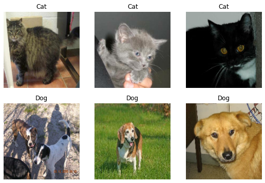
Let’s also examine how many of each class exist in the training data.
# Creates an iterator called labels
labels_iterator = train_dataset.unbatch().map(lambda image, label: label).as_numpy_iterator()

labels = [label for label in labels_iterator]
print("Cats:", labels.count(0))
print("Dogs:", labels.count(1))
Cats: 1000
Dogs: 1000
We can observe that the baseline machine learning model will have an accuracy of 50% since equal amounts of cats and dogs exist in the training data.
§2. First Model
Now, we can start by making our first basic model. By using the summary() method, we can view the number of parameters that will be trained in model1.
model1 = models.Sequential([
    # Convolutional Layers
    layers.Conv2D(16, (3, 3), activation = 'relu', input_shape = (160, 160, 3)),
    layers.MaxPooling2D((2, 2)),
    layers.Conv2D(16, (3, 3), activation = 'relu'),
    layers.MaxPooling2D((2, 2)),
    layers.Flatten(),

    # Fully Connected Layers
    layers.Dense(32, activation = 'relu'),
    layers.Dropout(0.2),
    layers.Dense(2, activation = 'softmax'),
])

model1.summary()
Model: "sequential"
_________________________________________________________________
 Layer (type)                Output Shape              Param #
=================================================================
 conv2d (Conv2D)             (None, 158, 158, 16)      448

 max_pooling2d (MaxPooling2D  (None, 79, 79, 16)       0
 )

 conv2d_1 (Conv2D)           (None, 77, 77, 16)        2320

 max_pooling2d_1 (MaxPooling  (None, 38, 38, 16)       0
 2D)

 flatten (Flatten)           (None, 23104)             0

 dense (Dense)               (None, 32)                739360

 dropout (Dropout)           (None, 32)                0

 dense_1 (Dense)             (None, 2)                 66

=================================================================
Total params: 742,194
Trainable params: 742,194
Non-trainable params: 0
_________________________________________________________________
We proceed by compiling model1 using Adam as our optimizer, Sparse Categorical Crossentropy as our loss, and accuracy as our performance measurement.
# Prepare model for training
model1.compile(optimizer='adam',
              loss=tf.keras.losses.SparseCategoricalCrossentropy(),
              metrics=['accuracy'])

# Train model
history1 = model1.fit(train_dataset,
                     epochs=20,
                     validation_data=validation_dataset)
Epoch 1/20
63/63 [==============================] - 15s 58ms/step - loss: 20.0576 - accuracy: 0.5075 - val_loss: 0.6944 - val_accuracy: 0.5000
Epoch 2/20
63/63 [==============================] - 4s 56ms/step - loss: 0.6882 - accuracy: 0.5000 - val_loss: 0.6941 - val_accuracy: 0.4864
Epoch 3/20
63/63 [==============================] - 4s 56ms/step - loss: 0.6827 - accuracy: 0.5295 - val_loss: 0.6992 - val_accuracy: 0.5136
Epoch 4/20
63/63 [==============================] - 4s 54ms/step - loss: 0.6562 - accuracy: 0.5935 - val_loss: 0.7230 - val_accuracy: 0.5136
Epoch 5/20
63/63 [==============================] - 4s 58ms/step - loss: 0.6387 - accuracy: 0.6210 - val_loss: 0.6975 - val_accuracy: 0.5260
Epoch 6/20
63/63 [==============================] - 4s 56ms/step - loss: 0.5961 - accuracy: 0.6680 - val_loss: 0.7231 - val_accuracy: 0.5495
Epoch 7/20
63/63 [==============================] - 4s 58ms/step - loss: 0.5706 - accuracy: 0.6930 - val_loss: 0.7357 - val_accuracy: 0.5755
Epoch 8/20
63/63 [==============================] - 4s 61ms/step - loss: 0.5270 - accuracy: 0.7410 - val_loss: 0.7293 - val_accuracy: 0.5854
Epoch 9/20
63/63 [==============================] - 4s 54ms/step - loss: 0.5106 - accuracy: 0.7475 - val_loss: 0.7640 - val_accuracy: 0.5780
Epoch 10/20
63/63 [==============================] - 4s 54ms/step - loss: 0.5083 - accuracy: 0.7585 - val_loss: 0.7489 - val_accuracy: 0.5767
Epoch 11/20
63/63 [==============================] - 4s 57ms/step - loss: 0.4736 - accuracy: 0.7850 - val_loss: 0.7996 - val_accuracy: 0.5755
Epoch 12/20
63/63 [==============================] - 4s 59ms/step - loss: 0.4611 - accuracy: 0.7850 - val_loss: 0.7386 - val_accuracy: 0.5792
Epoch 13/20
63/63 [==============================] - 4s 58ms/step - loss: 0.4268 - accuracy: 0.8185 - val_loss: 0.8819 - val_accuracy: 0.5804
Epoch 14/20
63/63 [==============================] - 4s 58ms/step - loss: 0.4176 - accuracy: 0.8155 - val_loss: 0.8698 - val_accuracy: 0.5842
Epoch 15/20
63/63 [==============================] - 4s 57ms/step - loss: 0.3944 - accuracy: 0.8235 - val_loss: 0.8576 - val_accuracy: 0.5879
Epoch 16/20
63/63 [==============================] - 4s 55ms/step - loss: 0.3742 - accuracy: 0.8245 - val_loss: 0.9501 - val_accuracy: 0.6114
Epoch 17/20
63/63 [==============================] - 4s 56ms/step - loss: 0.3443 - accuracy: 0.8400 - val_loss: 1.1005 - val_accuracy: 0.6101
Epoch 18/20
63/63 [==============================] - 4s 55ms/step - loss: 0.3368 - accuracy: 0.8420 - val_loss: 0.9829 - val_accuracy: 0.6040
Epoch 19/20
63/63 [==============================] - 4s 59ms/step - loss: 0.3105 - accuracy: 0.8465 - val_loss: 1.1383 - val_accuracy: 0.6114
Epoch 20/20
63/63 [==============================] - 4s 60ms/step - loss: 0.3063 - accuracy: 0.8530 - val_loss: 1.0984 - val_accuracy: 0.6064
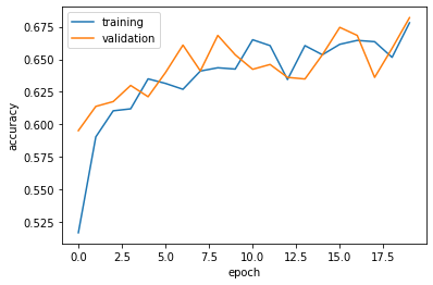
Let’s make a function to plot the accuracy.
def plot_history(hist):
    plt.plot(hist.history["accuracy"], label = "training")
    plt.plot(hist.history["val_accuracy"], label = "validation")
    plt.gca().set(xlabel = "epoch", ylabel = "accuracy")
    plt.legend()
    plt.show()

plot_history(history1)
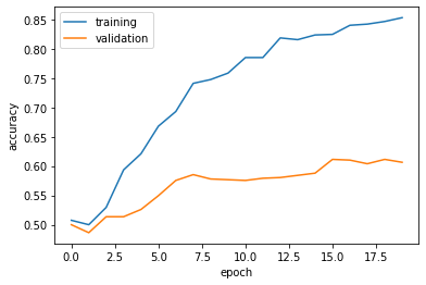
The validation accuracy of model1 stabilized around 58% during training. This is a bit better than the baseline. Overfitting can be observed since the training accuracy is around 93%, which is significantly higher than the validation accuracy.
§3. Model with Data Augmentation
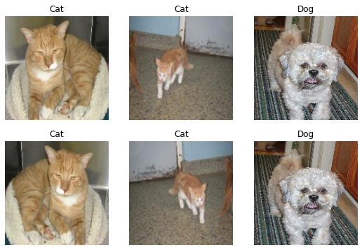
The previous model suffers from overfitting. A solution to this problem could be implementing data augmentation. In this post, we will utilize RandomFlip() and RandomRotation() layers. First, we can write a function to examine what these layers do to an image.
def plot_aug_examples(data, aug):
    plt.figure(figsize=(9, 6))
    for images, labels in data.take(1):
        # Take the first three images and apply the augmentation to them.
        imgs = aug(images[:3], training=True)
        lbls = tf.concat([labels[:3], labels[:3]], 0)
        imgs = tf.concat([images[:3], imgs], 0)
        for i in range(6):
            ax = plt.subplot(2, 3, i + 1)
            plt.imshow(imgs[i].numpy().astype("uint8"))
            plt.title(class_names[lbls[i]])
            plt.axis("off")
# Plot RandomFlip() examples
plot_aug_examples(train_dataset, layers.RandomFlip('horizontal'))
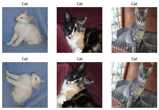
# Plot RandomRotation() examples
plot_aug_examples(train_dataset, layers.RandomRotation(1))
Now, let’s implement these layers into a new model.
model2 = models.Sequential([
    # Data Augmentation
    layers.RandomFlip('horizontal', input_shape = (160, 160, 3)),
    layers.RandomRotation(0.2),

    # Convolutional Layers
    layers.Conv2D(32, (3, 3), activation = 'relu'),
    layers.MaxPooling2D((2, 2)),
    layers.Conv2D(32, (3, 3), activation = 'relu'),
    layers.MaxPooling2D((2, 2)),
    layers.Flatten(),

    # Fully Connected Layers
    layers.Dense(64, activation = 'relu'),
    layers.Dropout(0.2),
    layers.Dense(2, activation = 'softmax'),
])

model2.summary()
Model: "sequential_1"
_________________________________________________________________
 Layer (type)                Output Shape              Param #
=================================================================
 random_flip_5 (RandomFlip)  (None, 160, 160, 3)       0

 random_rotation_5 (RandomRo  (None, 160, 160, 3)      0
 tation)

 conv2d_8 (Conv2D)           (None, 158, 158, 32)      896

 max_pooling2d_8 (MaxPooling  (None, 79, 79, 32)       0
 2D)

 conv2d_9 (Conv2D)           (None, 77, 77, 32)        9248

 max_pooling2d_9 (MaxPooling  (None, 38, 38, 32)       0
 2D)

 flatten_4 (Flatten)         (None, 46208)             0

 dense_7 (Dense)             (None, 64)                2957376

 dropout_5 (Dropout)         (None, 64)                0

 dense_8 (Dense)             (None, 2)                 130

=================================================================
Total params: 2,967,650
Trainable params: 2,967,650
Non-trainable params: 0
_________________________________________________________________
We compile the model with the same arguments.
# Prepare model for training
model2.compile(optimizer='adam',
              loss=tf.keras.losses.SparseCategoricalCrossentropy(),
              metrics=['accuracy'])

# Train model
history2 = model2.fit(train_dataset,
                      epochs=20,
                      validation_data=validation_dataset)
Epoch 1/20
63/63 [==============================] - 5s 58ms/step - loss: 44.8241 - accuracy: 0.5170 - val_loss: 0.6742 - val_accuracy: 0.5953
Epoch 2/20
63/63 [==============================] - 4s 57ms/step - loss: 0.6716 - accuracy: 0.5905 - val_loss: 0.6960 - val_accuracy: 0.6139
Epoch 3/20
63/63 [==============================] - 4s 56ms/step - loss: 0.6795 - accuracy: 0.6105 - val_loss: 0.6647 - val_accuracy: 0.6176
Epoch 4/20
63/63 [==============================] - 4s 57ms/step - loss: 0.6640 - accuracy: 0.6120 - val_loss: 0.6560 - val_accuracy: 0.6300
Epoch 5/20
63/63 [==============================] - 4s 55ms/step - loss: 0.6481 - accuracy: 0.6350 - val_loss: 0.6517 - val_accuracy: 0.6213
Epoch 6/20
63/63 [==============================] - 4s 55ms/step - loss: 0.6458 - accuracy: 0.6315 - val_loss: 0.6493 - val_accuracy: 0.6399
Epoch 7/20
63/63 [==============================] - 4s 56ms/step - loss: 0.6653 - accuracy: 0.6270 - val_loss: 0.6377 - val_accuracy: 0.6609
Epoch 8/20
63/63 [==============================] - 4s 55ms/step - loss: 0.6335 - accuracy: 0.6410 - val_loss: 0.6529 - val_accuracy: 0.6411
Epoch 9/20
63/63 [==============================] - 4s 56ms/step - loss: 0.6356 - accuracy: 0.6435 - val_loss: 0.6347 - val_accuracy: 0.6683
Epoch 10/20
63/63 [==============================] - 4s 57ms/step - loss: 0.6376 - accuracy: 0.6425 - val_loss: 0.6324 - val_accuracy: 0.6535
Epoch 11/20
63/63 [==============================] - 4s 62ms/step - loss: 0.6264 - accuracy: 0.6650 - val_loss: 0.6501 - val_accuracy: 0.6423
Epoch 12/20
63/63 [==============================] - 4s 57ms/step - loss: 0.6249 - accuracy: 0.6605 - val_loss: 0.6387 - val_accuracy: 0.6460
Epoch 13/20
63/63 [==============================] - 4s 56ms/step - loss: 0.6384 - accuracy: 0.6345 - val_loss: 0.6376 - val_accuracy: 0.6361
Epoch 14/20
63/63 [==============================] - 4s 57ms/step - loss: 0.6164 - accuracy: 0.6605 - val_loss: 0.6430 - val_accuracy: 0.6349
Epoch 15/20
63/63 [==============================] - 4s 55ms/step - loss: 0.6243 - accuracy: 0.6535 - val_loss: 0.6654 - val_accuracy: 0.6535
Epoch 16/20
63/63 [==============================] - 4s 57ms/step - loss: 0.6086 - accuracy: 0.6615 - val_loss: 0.6384 - val_accuracy: 0.6745
Epoch 17/20
63/63 [==============================] - 4s 61ms/step - loss: 0.6146 - accuracy: 0.6645 - val_loss: 0.6419 - val_accuracy: 0.6683
Epoch 18/20
63/63 [==============================] - 4s 57ms/step - loss: 0.6151 - accuracy: 0.6635 - val_loss: 0.6407 - val_accuracy: 0.6361
Epoch 19/20
63/63 [==============================] - 4s 57ms/step - loss: 0.6191 - accuracy: 0.6515 - val_loss: 0.6503 - val_accuracy: 0.6584
Epoch 20/20
63/63 [==============================] - 4s 57ms/step - loss: 0.6051 - accuracy: 0.6780 - val_loss: 0.6098 - val_accuracy: 0.6819
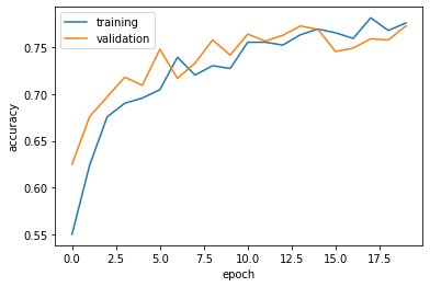
Here we can see a plot of the accuracy of model2.
plot_history(history2)
The validation accuracy of model2 stabilized between 63% and 68% during training. This is essentially the same as the accuracy from model1. Overfitting is not observed since the training accuracy is between 65% and 67%, which is similar to the validation accuracy.
§4. Data Preprocessing
Adding data augmentation successfully reduced overfitting, however the accuracy of the model is still not very good. The original data has pixels with RGB values between 0 and 255, but many models will train faster with RGB values normalized between 0 and 1, or possibly between -1 and 1. The following code will create a preprocessing layer called preprocessor which you can slot into your model pipeline.
# Preprocess images
i = tf.keras.Input(shape=(160, 160, 3))
x = tf.keras.applications.mobilenet_v2.preprocess_input(i)
preprocessor = tf.keras.Model(inputs = [i], outputs = [x])
Now, we add the preprocessor layer at the very beginning of our new model.
model3 = models.Sequential([
    preprocessor,

    # Data Augmentation Layers
    layers.RandomFlip('horizontal'),
    layers.RandomRotation(0.2),

    # Convolutional Layers
    layers.Conv2D(32, (3, 3), activation = 'relu'),
    layers.MaxPooling2D((2, 2)),
    layers.Conv2D(32, (3, 3), activation = 'relu'),
    layers.MaxPooling2D((2, 2)),
    layers.Flatten(),
    layers.Dropout(0.2),

    # Output Layer
    layers.Dense(2, activation = 'softmax'),
])

model3.summary()
Model: "sequential_2"
_________________________________________________________________
 Layer (type)                Output Shape              Param #
=================================================================
 model (Functional)          (None, 160, 160, 3)       0

 random_flip_2 (RandomFlip)  (None, 160, 160, 3)       0

 random_rotation_2 (RandomRo  (None, 160, 160, 3)      0
 tation)

 conv2d_4 (Conv2D)           (None, 158, 158, 32)      896

 max_pooling2d_4 (MaxPooling  (None, 79, 79, 32)       0
 2D)

 conv2d_5 (Conv2D)           (None, 77, 77, 32)        9248

 max_pooling2d_5 (MaxPooling  (None, 38, 38, 32)       0
 2D)

 flatten_2 (Flatten)         (None, 46208)             0

 dropout_2 (Dropout)         (None, 46208)             0

 dense_4 (Dense)             (None, 2)                 92418

=================================================================
Total params: 102,562
Trainable params: 102,562
Non-trainable params: 0
_________________________________________________________________
We compile model3 with the same arguments as the previous models.
# Prepare model for training
model3.compile(optimizer='adam',
              loss=tf.keras.losses.SparseCategoricalCrossentropy(),
              metrics=['accuracy'])

# Train model
history3 = model3.fit(train_dataset,
                      epochs=20,
                      validation_data=validation_dataset)
Epoch 1/20
63/63 [==============================] - 5s 58ms/step - loss: 0.7206 - accuracy: 0.5505 - val_loss: 0.6320 - val_accuracy: 0.6250
Epoch 2/20
63/63 [==============================] - 4s 55ms/step - loss: 0.6353 - accuracy: 0.6240 - val_loss: 0.6027 - val_accuracy: 0.6757
Epoch 3/20
63/63 [==============================] - 4s 55ms/step - loss: 0.6036 - accuracy: 0.6755 - val_loss: 0.5946 - val_accuracy: 0.6968
Epoch 4/20
63/63 [==============================] - 4s 62ms/step - loss: 0.5976 - accuracy: 0.6900 - val_loss: 0.5684 - val_accuracy: 0.7178
Epoch 5/20
63/63 [==============================] - 4s 55ms/step - loss: 0.5761 - accuracy: 0.6955 - val_loss: 0.5734 - val_accuracy: 0.7092
Epoch 6/20
63/63 [==============================] - 4s 56ms/step - loss: 0.5663 - accuracy: 0.7045 - val_loss: 0.5336 - val_accuracy: 0.7475
Epoch 7/20
63/63 [==============================] - 5s 80ms/step - loss: 0.5331 - accuracy: 0.7390 - val_loss: 0.5529 - val_accuracy: 0.7166
Epoch 8/20
63/63 [==============================] - 5s 65ms/step - loss: 0.5354 - accuracy: 0.7200 - val_loss: 0.5244 - val_accuracy: 0.7327
Epoch 9/20
63/63 [==============================] - 4s 59ms/step - loss: 0.5350 - accuracy: 0.7300 - val_loss: 0.4930 - val_accuracy: 0.7574
Epoch 10/20
63/63 [==============================] - 4s 57ms/step - loss: 0.5184 - accuracy: 0.7270 - val_loss: 0.5268 - val_accuracy: 0.7413
Epoch 11/20
63/63 [==============================] - 4s 56ms/step - loss: 0.5044 - accuracy: 0.7550 - val_loss: 0.5142 - val_accuracy: 0.7636
Epoch 12/20
63/63 [==============================] - 4s 57ms/step - loss: 0.5009 - accuracy: 0.7550 - val_loss: 0.5102 - val_accuracy: 0.7562
Epoch 13/20
63/63 [==============================] - 4s 57ms/step - loss: 0.5016 - accuracy: 0.7520 - val_loss: 0.4981 - val_accuracy: 0.7624
Epoch 14/20
63/63 [==============================] - 4s 57ms/step - loss: 0.4857 - accuracy: 0.7630 - val_loss: 0.4940 - val_accuracy: 0.7723
Epoch 15/20
63/63 [==============================] - 4s 57ms/step - loss: 0.4874 - accuracy: 0.7690 - val_loss: 0.5018 - val_accuracy: 0.7686
Epoch 16/20
63/63 [==============================] - 4s 56ms/step - loss: 0.4858 - accuracy: 0.7650 - val_loss: 0.5046 - val_accuracy: 0.7450
Epoch 17/20
63/63 [==============================] - 4s 57ms/step - loss: 0.4859 - accuracy: 0.7590 - val_loss: 0.5009 - val_accuracy: 0.7488
Epoch 18/20
63/63 [==============================] - 4s 56ms/step - loss: 0.4689 - accuracy: 0.7810 - val_loss: 0.5218 - val_accuracy: 0.7587
Epoch 19/20
63/63 [==============================] - 4s 55ms/step - loss: 0.4800 - accuracy: 0.7675 - val_loss: 0.5147 - val_accuracy: 0.7574
Epoch 20/20
63/63 [==============================] - 4s 55ms/step - loss: 0.4825 - accuracy: 0.7755 - val_loss: 0.5114 - val_accuracy: 0.7723
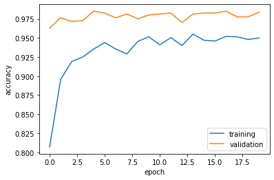
Here we can see a plot of the accuracy of model3.
plot_history(history3)
The validation accuracy of model3 stabilized between 74% and 77% during training. This is significantly better than the accuracy from model2. Overfitting is not observed since the training accuracy stabilized between 75% and 78%, which is similar to the validation accuracy.
§5. Transfer Learning
The performance of model3 is decent, but we can do better. So far, we’ve been training models for distinguishing between cats and dogs from scratch. In some cases, however, someone might already have trained a model that does a related task, and might have learned some relevant patterns. We could use a pre-existing model for our task. To do this, we need to first access a pre-existing “base model”, incorporate it into a full model for our current task, and then train that model.
Use the following code in order to download MobileNetV2 and configure it as a layer that can be included in your model.
IMG_SHAPE = IMG_SIZE + (3,)
base_model = tf.keras.applications.MobileNetV2(input_shape=IMG_SHAPE,
                                               include_top=False,
                                               weights='imagenet')
# Prevent existing parameters from being updated during training
base_model.trainable = False

i = tf.keras.Input(shape=IMG_SHAPE)
x = base_model(i, training = False)
base_model_layer = tf.keras.Model(inputs = [i], outputs = [x])
Downloading data from https://storage.googleapis.com/tensorflow/keras-applications/mobilenet_v2/mobilenet_v2_weights_tf_dim_ordering_tf_kernels_1.0_160_no_top.h5
9412608/9406464 [==============================] - 0s 0us/step
9420800/9406464 [==============================] - 0s 0us/step
To create model4, we remove our old convolutional layers and replace them with the MobileNetV2 layer.
model4 = models.Sequential([
    preprocessor,

    # Data Augmentation Layers
    layers.RandomFlip('horizontal'),
    layers.RandomRotation(0.2),

    # Transfer Learning Layer
    base_model_layer,
    layers.GlobalMaxPooling2D(),
    layers.Dropout(0.2),

    # Output Layer
    layers.Dense(2, activation = 'softmax'),
])

model4.summary()
Model: "sequential_3"
_________________________________________________________________
 Layer (type)                Output Shape              Param #
=================================================================
 model (Functional)          (None, 160, 160, 3)       0

 random_flip_3 (RandomFlip)  (None, 160, 160, 3)       0

 random_rotation_3 (RandomRo  (None, 160, 160, 3)      0
 tation)

 model_1 (Functional)        (None, 5, 5, 1280)        2257984

 global_max_pooling2d (Globa  (None, 1280)             0
 lMaxPooling2D)

 dropout_3 (Dropout)         (None, 1280)              0

 dense_5 (Dense)             (None, 2)                 2562

=================================================================
Total params: 2,260,546
Trainable params: 2,562
Non-trainable params: 2,257,984
_________________________________________________________________
Here, we note that while there are a lot of parameters, only 2,562 are trainable.
We compile model4 the same way as the other models.
# Prepare model for training
model4.compile(optimizer='adam',
              loss=tf.keras.losses.SparseCategoricalCrossentropy(),
              metrics=['accuracy'])

# Train model
history4 = model4.fit(train_dataset,
                      epochs=20,
                      validation_data=validation_dataset)
Epoch 1/20
63/63 [==============================] - 8s 82ms/step - loss: 0.7795 - accuracy: 0.8070 - val_loss: 0.1443 - val_accuracy: 0.9629
Epoch 2/20
63/63 [==============================] - 4s 62ms/step - loss: 0.3914 - accuracy: 0.8955 - val_loss: 0.0719 - val_accuracy: 0.9765
Epoch 3/20
63/63 [==============================] - 4s 61ms/step - loss: 0.3050 - accuracy: 0.9190 - val_loss: 0.0797 - val_accuracy: 0.9715
Epoch 4/20
63/63 [==============================] - 4s 62ms/step - loss: 0.2766 - accuracy: 0.9250 - val_loss: 0.0683 - val_accuracy: 0.9728
Epoch 5/20
63/63 [==============================] - 4s 63ms/step - loss: 0.2263 - accuracy: 0.9355 - val_loss: 0.0498 - val_accuracy: 0.9851
Epoch 6/20
63/63 [==============================] - 4s 62ms/step - loss: 0.2216 - accuracy: 0.9440 - val_loss: 0.0487 - val_accuracy: 0.9827
Epoch 7/20
63/63 [==============================] - 4s 64ms/step - loss: 0.2495 - accuracy: 0.9355 - val_loss: 0.0728 - val_accuracy: 0.9765
Epoch 8/20
63/63 [==============================] - 4s 63ms/step - loss: 0.2540 - accuracy: 0.9290 - val_loss: 0.0526 - val_accuracy: 0.9814
Epoch 9/20
63/63 [==============================] - 4s 63ms/step - loss: 0.1976 - accuracy: 0.9455 - val_loss: 0.0824 - val_accuracy: 0.9752
Epoch 10/20
63/63 [==============================] - 4s 62ms/step - loss: 0.1713 - accuracy: 0.9515 - val_loss: 0.0538 - val_accuracy: 0.9802
Epoch 11/20
63/63 [==============================] - 4s 64ms/step - loss: 0.2004 - accuracy: 0.9410 - val_loss: 0.0548 - val_accuracy: 0.9814
Epoch 12/20
63/63 [==============================] - 4s 62ms/step - loss: 0.2102 - accuracy: 0.9505 - val_loss: 0.0535 - val_accuracy: 0.9827
Epoch 13/20
63/63 [==============================] - 4s 64ms/step - loss: 0.2105 - accuracy: 0.9400 - val_loss: 0.0920 - val_accuracy: 0.9703
Epoch 14/20
63/63 [==============================] - 4s 62ms/step - loss: 0.1517 - accuracy: 0.9550 - val_loss: 0.0437 - val_accuracy: 0.9814
Epoch 15/20
63/63 [==============================] - 4s 65ms/step - loss: 0.1815 - accuracy: 0.9470 - val_loss: 0.0507 - val_accuracy: 0.9827
Epoch 16/20
63/63 [==============================] - 4s 67ms/step - loss: 0.2071 - accuracy: 0.9460 - val_loss: 0.0565 - val_accuracy: 0.9827
Epoch 17/20
63/63 [==============================] - 4s 63ms/step - loss: 0.1852 - accuracy: 0.9520 - val_loss: 0.0400 - val_accuracy: 0.9851
Epoch 18/20
63/63 [==============================] - 4s 64ms/step - loss: 0.1627 - accuracy: 0.9515 - val_loss: 0.0750 - val_accuracy: 0.9777
Epoch 19/20
63/63 [==============================] - 4s 65ms/step - loss: 0.1669 - accuracy: 0.9480 - val_loss: 0.0686 - val_accuracy: 0.9777
Epoch 20/20
63/63 [==============================] - 4s 64ms/step - loss: 0.1645 - accuracy: 0.9500 - val_loss: 0.0477 - val_accuracy: 0.9839
Here we can see a plot of the accuracy of model4.
plot_history(history4)
The validation accuracy of model4 stabilized around 98% during training. This is significantly better than the accuracy from model3. Overfitting is not observed since the training accuracy stabilized around 95%, which is similar to the validation accuracy.
§6. Score on Test Data
Based on all of the validation accuracies, model4 is the best performer. Let’s evaluate its performance on the unseen test data.
# Evaluate model on test data
loss, accuracy = model4.evaluate(test_dataset)
print('Test accuracy :', accuracy)
6/6 [==============================] - 1s 49ms/step - loss: 0.0563 - accuracy: 0.9896
Test accuracy : 0.9895833134651184
Using model4, we get an accuracy of about 99% on the test data. This is great since it also matches the test and validation accuracies.