In this project, we designed and trained an Artificial Neural Network (ANN) that can be used to make predictions on a specified stock ticker.

Here’s a link to our project repository:

https://github.com/acgowda/market-flow

We extracted live data and performed data cleaning, encoding, and normalization.

Then, we trained our model using Tensorflow and Keras on Google Colab and data from Yahoo Finance on the weekly price changes of all the stocks in the S&P 500.

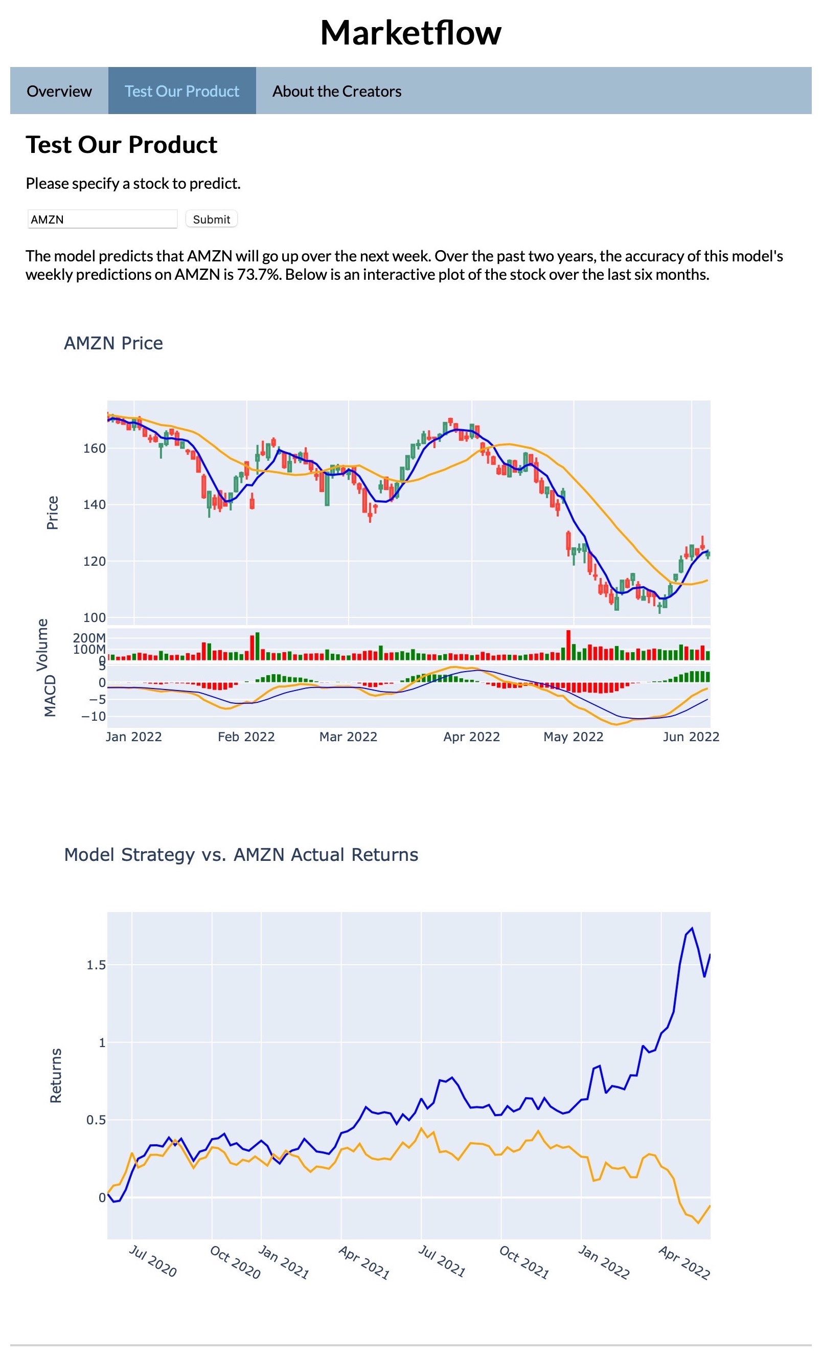
We also deployed our model using a Flask web app. This app allows users to input a desired stock, and outputs a prediction for the next week, as well as an interactive plot that displays the model’s performance on the most recent 6 months of data. Another plot displays the model’s net profit over two years when using it to make trades and compares it to the actual returns. The details of this web app can be viewed in the app folder. To run the web app locally, clone the repo and run flask run.

Finally, we published our app onto the web using Heroku. See https://market-flow.herokuapp.com

Data Processing

The first step of our project involved performed data collection and processing. This is all done within the get_data.py file.

To begin, we built a function called get_sp500_tickers() to get a list of ticker symbols for stocks in the S&P 500 index. We then feed this list of tickers into a function called get_input_data(), which relies on several functions nested within each other to perform the following:

1. Obtain our data from yahoo finance.
2. Merge different datasets together to build our feature space.
3. Normalize the data by converting columns from raw price or volume data to percentage change data.
4. Create moving average features.
5. Deal with NaN and infinite vlaues.
6. Create our target variable.
7. Create temporal indicator variables.
8. Shuffle our data appropriately.
9. Ensure that our binary classification task is balanced (i.e. target feature contains an equal number of buy and sell signals).

We also implemented a certain level of flexibility into the get_input_data() function, allowing the user to specify whether they want weekly or daily observations in their training set; the number of moving average columns they want to add to their feature space; the index and commodity pricing and volumne information that they wanted to add to their feature-space; and the period over which they wanted their information to come from.

With this function, we were able to train a successful ANN.

Meanwhile, we created a separate function called get_preds_data() to obtain our prediction data (i.e. the data we used to generate model prediction and returns statistics on our website). This function has a lot of similarities with get_input_data(). However, some key differences are that get_preds_data() only accepts 1 ticker and that the data is no longer shuffled because we want to preserve the order of our series when plotting it (note that this doesn’t imply that the order matters for making predictions).

Function for getting list of most recent S&P 500 tickers

def get_sp500_tickers():
    """
    Returns a data frame of the most recent
    S&P 500 tickers from the Wikipedia page
    on the S&P 500 Index

    Also saves a pickle file of the tickers for future use
    """
    tickers = pd.read_html(
    'https://en.wikipedia.org/wiki/List_of_S%26P_500_companies')[0]['Symbol']

    with open('sp500_tickers','wb') as f:
        pickle.dump(tickers,f)
    return tickers

Function for getting our training data

def get_input_data(tickers,indices = ["^GSPC","^VIX"],
                   period = '5y',
                   resolution = '1d',
                   MAs = [5,20,60,200]):
    """
    Gets the data we need for model training or testing;
    Ensures that the dataset has equal number of buy/sell signals
    in it, so that our model training and testing process won't
    be biased

    Indices will default to "^GSPC","^VIX" which
    represent the S&P500 index and VIX index on
    yahoo finance, respectively
    """
    df = compile_data(tickers,indices,period,resolution,MAs)

    # obtain whichever is lower: the number of buy signals (1)
    # or the number of sell signals (0)
    lower = min(len(df.loc[df['close'] == 1]), len(df.loc[df['close'] == 0]))

    # balance our data: 
      # get dataframes of buys and sells which have the same number
      # of buy and sell signals
      # and combine them into a single dataframe
    # i.e. downsample whichever has more obs
    buys_df = df.loc[df['close'] == 1].sample(frac=lower/len(df.loc[df['close'] == 1]))
    sells_df = df.loc[df['close'] == 0].sample(frac=lower/len(df.loc[df['close'] == 0]))
    df_new = pd.concat([buys_df,sells_df],axis = 0)

    # shuffle the data
    df_new = df_new.sample(frac = 1)

    return df_new

Function for getting prediction data

def get_preds_data(ticker,indices = ["^GSPC","^VIX"],
                   period = '4y',
                   resolution = '1d',
                   MAs = [5,20,60,200]):
    """
    Get data for model to make predictions on
    """
    # yahoo finance doesn't like '.' full stops, and prefers '-' dashes
    ticker = ticker.replace('.', '-')
    # read in a specific ticker's historical financial information
    df = yf.Ticker(ticker).history(period = period,interval = resolution)
    index_df = get_index_data(indices,period,resolution,MAs)

    # drop columns we won't be using from that dataframe
    df.drop(['Dividends','Stock Splits'],axis = 1,inplace = True)
    # make column names lower cased, because it's easier to type
    for col in df.columns:
        df.rename(columns = {col:col.lower()},inplace = True)

    # drop NAs for jic
    df.dropna(inplace = True)
    
    # add a few rolling window columns on our closing price
    df = create_close_MAs(df,MAs)
    
    # normalise all columns as percentages
    df = df.pct_change()

    # fill foward missing values just in case any came up
    df.fillna(method = 'ffill')

    df = remove_inf(df) # remove inf values

    df = pd.concat([df,index_df], axis=1, ignore_index=False)

    df['returns'] = df['close']
    # merge the extra financial info along the column-axis
    df = create_target(df)

    # get day of week; 0 = Monday, ..., so on so forth
    # as a column
    if resolution == '1d':
      df['day'] = list(pd.Series(df.index).apply(lambda x: str(x.weekday())))

    # get month of year as a column
    df['month'] = list(pd.Series(df.index).apply(lambda x: str(x.month)))

    # convert categorical data to dummy variables
    df = pd.get_dummies(df)

    df.dropna(inplace=True)

    return df

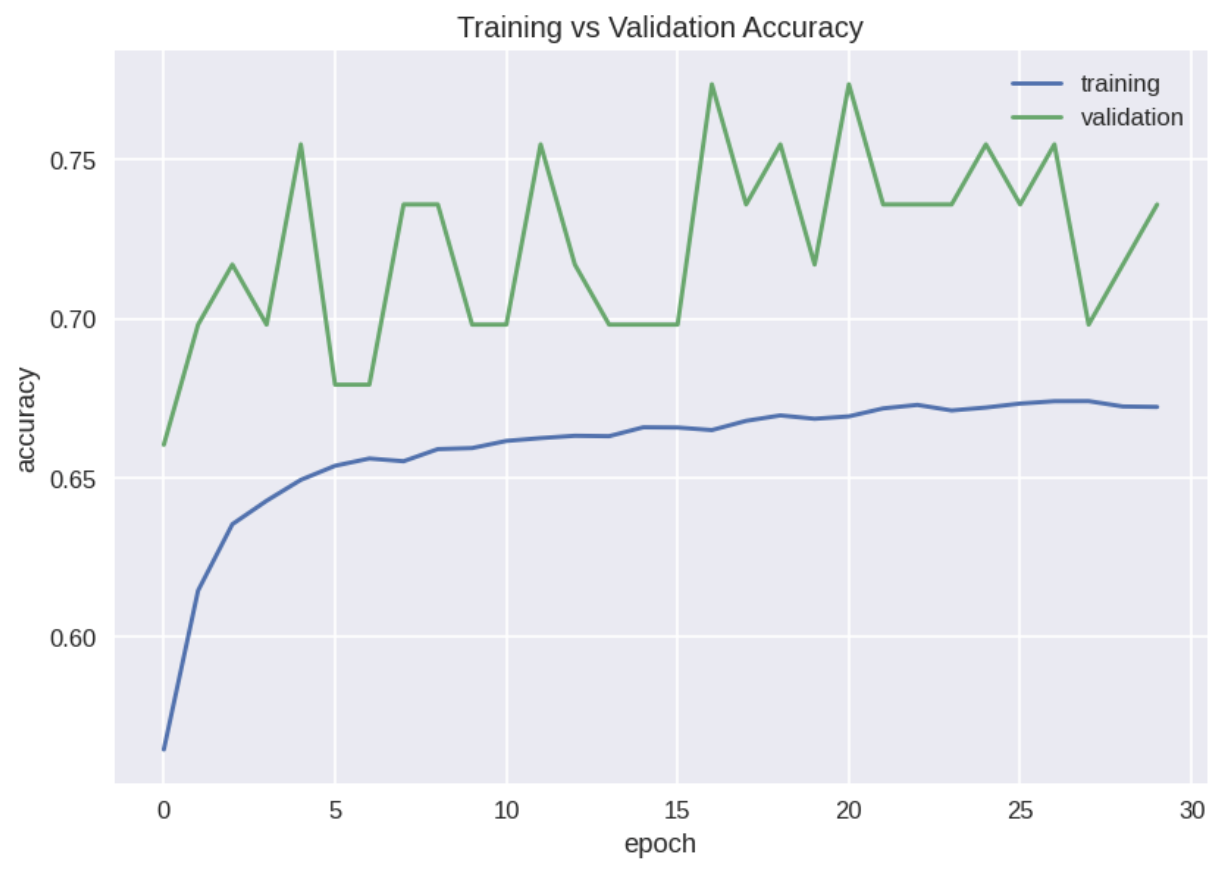
Model Training

Now, we build and train our model. You can view the details in model/model_testing.ipynb. Reading in the .csv file, the dataframe gives stock data with the following columns:

['Date', 'open', 'high', 'low', 'close', 'volume', 'ma4', 'ma21', 'ma52',
 '^GSPC-close', '^GSPC-volume', '^GSPC-ma4', '^GSPC-ma21', '^GSPC-ma52',
 '^VIX-close', '^VIX-ma4', '^VIX-ma21', '^VIX-ma52', '^IXIC-close',
 '^IXIC-volume', '^IXIC-ma4', '^IXIC-ma21', '^IXIC-ma52', '^DJI-close',
 '^DJI-volume', '^DJI-ma4', '^DJI-ma21', '^DJI-ma52', '^HSI-close',
 '^HSI-volume', '^HSI-ma4', '^HSI-ma21', '^HSI-ma52', '^FTSE-close',
 '^FTSE-volume', '^FTSE-ma4', '^FTSE-ma21', '^FTSE-ma52', '^FCHI-close',
 '^FCHI-volume', '^FCHI-ma4', '^FCHI-ma21', '^FCHI-ma52', 'GC=F-close',
 'GC=F-volume', 'GC=F-ma4', 'GC=F-ma21', 'GC=F-ma52', 'CL=F-close',
 'CL=F-volume', 'CL=F-ma4', 'CL=F-ma21', 'CL=F-ma52', 'month_1',
 'month_10', 'month_11', 'month_12', 'month_2', 'month_3', 'month_4',
 'month_5', 'month_6', 'month_7', 'month_8', 'month_9']

The ‘close’ column is separated as the target variable, and the rest of the columns are used as predictor variables. We create our ANN with a Keras Sequential model:

model = tf.keras.models.Sequential([
    layers.Dense(128, input_shape=(61,), activation='relu'),
    layers.Dropout(0.2),
    layers.Dense(128, activation='relu'),
    layers.Dropout(0.2),
    layers.Dense(64, activation='relu'),
    layers.Dropout(0.2),
    layers.Dense(2)
])

and train it over 30 epochs. The training history is shown below.

We save the model to be used in the web app using model.save().

Flask App

Finally, we deployed our code onto a web app via Flask. The app folder contains the __init__.py file which initializes the web app, a templates folder containing html files that are rendered by Flask, and a static folder containing styling and a favicon for the web app.

First, we create the Flask app:

from flask import Flask
app = Flask(__name__)

We use regular routing to describe the behavior of the web app when accessing various pages:

@app.route('/')
def main():
    return render_template('main.html')

@app.route('/about/')
def about():
    return render_template('about.html')

These render the main.html and about.html files found in the templates folder. In particular, our html uses Jinja, which allows for html files to extend a ‘base’ file, as well as convenient parsing of Python variables. You can read more about Jinja here.

Our implementation of the test() function performs a POST request to retrieve the user’s desired stock and makes a prediction on this stock, as well as evaluates the model on the past 6 months. Then, it uses the plot_ticker() and plot_returns() functions in the plot_data.py file which build and return prediction and returns plots. We use JSON encoding to process the figure and render it with Flask along with the test.html file.

The following code is needed to encode each figure:

tickerJSON = json.dumps(plot_ticker(df, target), cls=plotly.utils.PlotlyJSONEncoder)

and to insert them into the html:

<div id='chart' class='chart'></div>
<script src='https://cdn.plot.ly/plotly-latest.min.js'></script>
<script type='text/javascript'>
  var graphs = ;
  Plotly.plot('chart',graphs,{});
</script>

Here is a screenshot of the test.html page after a user makes a submission:

Conclusion

In this project, we succeeded at building a neural network that could accurately predict the up or down movement of the closing price of various financial securities. However, our model’s returns are not very good. One reason that may be the case is that our model is good at picking up smaller movements (e.g. up/down price movement of <= 1%) than it is at registering larger movements (e.g. up/down price movement of > 3%). This means that although we have a generally high accuracy, we have a higher chance of losing on the worst days and not gaining on the best days, which can greatly affect financial performance beyond model accuracy.

We can solve this problem by changing our target variable or adjusting our portfolio weights when we run the strategy. More specifically, we can change our target variable to indicate when there is a significant up week, significant down week, and when there are no significant weekly changes. By doing so, we can get more accurate recommendations from our model, which might improve our investment performance. Otherwise, we can simply adjust the amount we invest based on the model’s confidence in its prediction. For instance, we invest less in our model’s recommendation when it is less confident in its prediction, and we can invest more when the model is more confident in its prediction.

References:

https://python.plainenglish.io/a-simple-guide-to-plotly-for-plotting-financial-chart-54986c996682 https://pythonprogramming.net/cryptocurrency-recurrent-neural-network-deep-learning-python-tensorflow-keras/